Whistler-induced electron precipitation from the Van Allen radiation belts occurs as a result of coupling between the troposphere and the magnetosphere. For some electron energy ranges Whistler-induced Electron Precipitation (WEP) is a significant inner radiation belt loss process [e.g., Dungey, 1963; Rodger et al., 2003], acting as one of the drivers by which whistler mode waves (e.g., plasmaspheric hiss, lightning-generated whistlers) cause pitch angle scattering. The energetic electron precipitation arises from lightning produced whistlers [Storey, 1953] interacting with cyclotron resonant radiation belt electrons near the equatorial zone [Tsurutani and Lakhina, 1997]. Pitch angle scattering of energetic radiation belt electrons [Kennel and Petschek, 1966] by whistler mode waves drives some resonant electrons into the bounce loss cone, resulting in their precipitation into the atmosphere [Rycroft, 1973]. A schematic of WEP is shown in Figure 1.
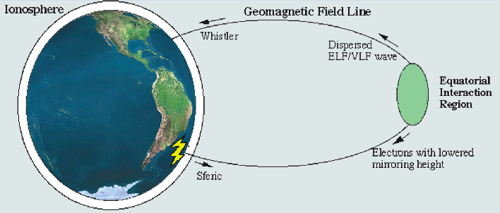
Figure 1. Schematic of whistler induced electron precipitation (WEP) (adapted from Rodger [1999]).
At this time reports on in-situ satellite measurements of WEP losses are fairly rare. S81-1 satellite measurements in the energy range from 6-950 keV have reported short bursts (~0.2 s) of magnetically guided and focused electrons in the bounce loss cone, primarily in the range ~75 to ~300 keV. A total of 15 WEP events were found to be correlated on a one-to-one basis with single-hop whistlers observed at Palmer, Antarctica [Voss et al., 1998], while the several hundred WEP events observed were correlated with active lightning. These WEP events were found to be globally correlated with regions of high lightning activity, principally in the range 2<L<3. A portion of the WEP electrons were observed to backscatter from the atmosphere and bounce repeatedly between the northern and southern hemispheres, leading to a series of decreasing WEP bursts into both hemispheres over a period of ~2-3 s. Most recently, SAMPEX and UARS satellite data have revealed hundreds of cases where enhanced losses of 100-200 keV electrons were associated with individual thunderstorms [Blake et al., 2001]. The latter authors have argued that the extensive amount of observed precipitation suggests that WEP, driven by global thunderstorm activity, may be a significant factor in controlling the lifetime of energetic electrons in the inner belt and slot regions.
An important parameter for determining the overall importance of WEP to radiation belt losses is the magnitude of a “typical” WEP event. This may be calculated from theoretical studies [e.g., Abel and Thorne, 1998] or inferred from experimental observations, such as in-situ measurements of WEP events [Voss et al., 1998]. Recently, a different approach has been to use experimental observations to characterize typical WEP magnitudes. Combining reports of satellite WEP observations with ground based whistler measurements, Rodger et al. [2005] showed that the precipitation of energetic electrons by these bursts in the range L=1.9-3.5 will lead to a mean rate of energy deposited into the atmosphere of 3×10⁻⁴ ergs cm-2 min-1.
It is expected that the spatial distribution of WEP events will vary in a similar manner to the distribution of lightning activity, albeit when expressed in geomagnetic coordinates. Figure 2 shows the annual average global total lightning activity in Corrected GeoMagnetic (CGM) coordinates based on the Definite/International Geomagnetic Reference Field (DGRF/IGRF) for 2003 at 100 km altitude, using the GEOPACK software routines. To aid the eye, this figure shows the geographical coastlines also translated into CGM coordinates. Lightning activity has been suppressed on this plot for very low latitudes (<5º), where the GEOPACK calculation is not reliable. This is unlikely to influence any of the following conclusions, as the coupling of lightning activity to WEP is dependent upon geomagnetic latitude, and hence L. In situ observations indicate that WEP is rare at low L-shells [Voss et al., 1998], despite high lightning activity (Figure 1), due to increasingly unfavourable gyroresonance conditions [Friedel and Hughes, 1992]. This L-variation in this coupling can be reasonably estimated from SEEP measurements of how experimentally observed WEP varies with L [Figure 11, Voss et al., 1998].

Figure 2. The annual average global total lightning activity (in units of flashes km-2 yr-1) transformed into CGM geomagnetic co-ordinates (after Rodger et al. [2005]).
Combining existing knowledge of this coupling parameter, typical lightning activity (Figure 2), and the dependence of WEP precipitation fluxes on the strength of the associated lightning’s return stroke peak current has been identified [Clilverd et al., 2004], an estimate of the spatially variation in WEP energy deposition into the atmosphere has been published [Rodger et al., 2005], as shown in Figure 3.
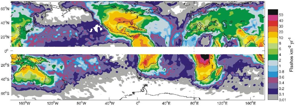
Figure 3. Map showing the expected global distribution in the rate of energy deposited by WEP into the atmosphere (after Rodger et al. [2005]).
The rate of energy deposited by WEP into the atmosphere is higher for the northern hemisphere than the southern, as expected from the variation in lightning activity (Figure 2). This results in the mean WEP energy input rate for all longitudes at L~2.3 in this northern hemisphere being almost twice that for the southern hemisphere (8×10⁻⁴ ergs cm-2 min-1 c.f. 4.7×10⁻⁴ ergs cm-2 min-1). The strongest energy inputs occur over North America, as expected by the high lightning activity occurring in this region at high geomagnetic latitudes [Rodger et al., Fig. 1, 2004a]. Nonetheless, most of the global lightning will not generate WEP, as it occurs in the 3 tropical “chimney” regions of tropical America and Africa, and the Maritime Continent (SE Asia and northern Australia and the Indonesian archipelago) [Christian et al.,Fig. 4., 2003]. Because of the coupling between lightning and observed WEP (Section 2.3), virtually all of the energy deposited by WEP occurs in the bands shown in Figures 3 and 7. The mean rate of energy deposited by WEP into the atmosphere inside these bands is 3×10⁻⁴ ergs cm-2 min-1, varying from a low of zero to the North American high of 5.6×10⁻³ ergs cm-2 min-1.
The typical energy range of the electrons precipitated by a WEP burst penetrates into the atmosphere to altitudes of 60-85 km, the ionospheric D-region. This is one of the least well understood parts of the atmosphere. There is currently a fairly poor understanding of the properties, creation, and variability of this region. One complementary technique to study WEP makes use of long range remote sensing of very low frequency (VLF) waves propagating inside the waveguide bounded by the lower ionosphere and the Earth’s surface. Significant variations in the received amplitude and/or phase of fixed frequency VLF transmissions arise from localized changes in the lower ionosphere. Further discussion on the use of subionospheric VLF propagation as a remote sensing probe can be found in recent review articles [e.g., Barr et al., 2000; Rodger, 2003]. WEP leads to localized ionospheric modifications produced by secondary ionisation just below the D-region of the ionosphere, which are observed as “Trimpi” perturbations in subionospheric VLF transmissions [Helliwell et al., 1973].Examples of Trimpi perturbations in amplitude and phase are shown in Figures 4 and 5. These perturbations begin with a relatively fast (~1 s) change in the received amplitude and/or phase, followed by a slower relaxation (< 100 s) back to the unperturbed signal level due to the recombination of the additional ionisation. Trimpi perturbations permit observers to study WEP fluxes and the chemistry of the nighttime lower ionosphere [e.g., Pasko and Inan, 1994], from locations remote from the actual precipitation region.
Until recently there was considerable uncertainty as to the typical size of the D-region patch altered by WEP. Trimpi perturbations have been used to show that WEP produced patches are large (at least 600 km´1500 km) [Clilverd et al., 2002], considerably larger than the observed dimensions of whistler ducts [e.g., Angerami, 1970]. Large D-region patch dimensions have been explained through a quasi-trapped whistler propagation theory in which ducted energy spreads at the magnetic equator [Strangeways, 1999], resulting in whistler-mode signals which have leaked outside their whistler duct still contributing to the horizontal lateral extent of WEP. Such leakage would give a significantly larger precipitation footprint than the actual dimensions of the whistler duct. A different mechanism also leading to large WEP patch dimensions comes through the precipitation caused by obliquely (nonducted) propagating whistlers, creating an ionospheric disturbance of ~1000 km spatial extent [Johnson et al., 1999]. At this stage there is no clear experimental evidence to indicate whether quasi-ducted or nonducted whistler propagation dominates the overall WEP losses [Rodger et al., 2003].
The decay timescale information from Trimpi signatures has been used to determine the vertical dimensions of the WEP modified ionospheric patches. An analysis of 134 Trimpis observed at Palmer station (Antarctica) on transmissions from NPM (Hawaii) reported that the “recovery signatures” (decay) could be approximated by an exponential function for the purposes of determining the decay rate [Pasko and Inan, 1994]. A later report concluded that the decay of Trimpis follow a logarithmic dependence [Dowden et al., 2001], noting that the difference between exponential decay and logarithmic decay is relatively small except near the beginning (near onset) and end of the perturbation. This study also noted that a re-examination of Trimpi observed in Tokyo from NWC (Australia), were also consistent with a logarithmic decay signature, rather than exponential decay with two characteristic time scales, as originally concluded [Molchanov et al., 1998].
A number of theoretical studies have made use of electron density perturbations with a vertical Gaussian profile to represent the WEP produced ionospheric electron density modification [Nunn and Strangeways, 2000; Clilverd et al., 2002], while others have studied modifications derived from satellite observed WEP fluxes [e.g., Pasko and Inan, 1994; Rodger et al., 2002]. For example, it has been reported that the observed Trimpi recovery signatures may be used to determine the energy content of WEP bursts [Pasko and Inan, 1994].
Figure 4. Example of a classic Trimpi perturbation in amplitude and phase observed on transmissions from the US Navy transmitter NPM at Faraday (Antarctica) on 23 April 1994 (after Dowden et al. [2001]).
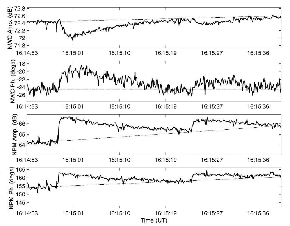
Figure 5. An example of a fairly large Trimpi event observed on transmissions from NWC and NPM at Dunedin on 1 November 2003. The time resolution is 0.4 s. The unperturbed behaviour of the signals is indicated by the long dashed lines (after Rodger et al. [2005]).
References
References for the papers cited in this background material piece are listed together on another webpage.